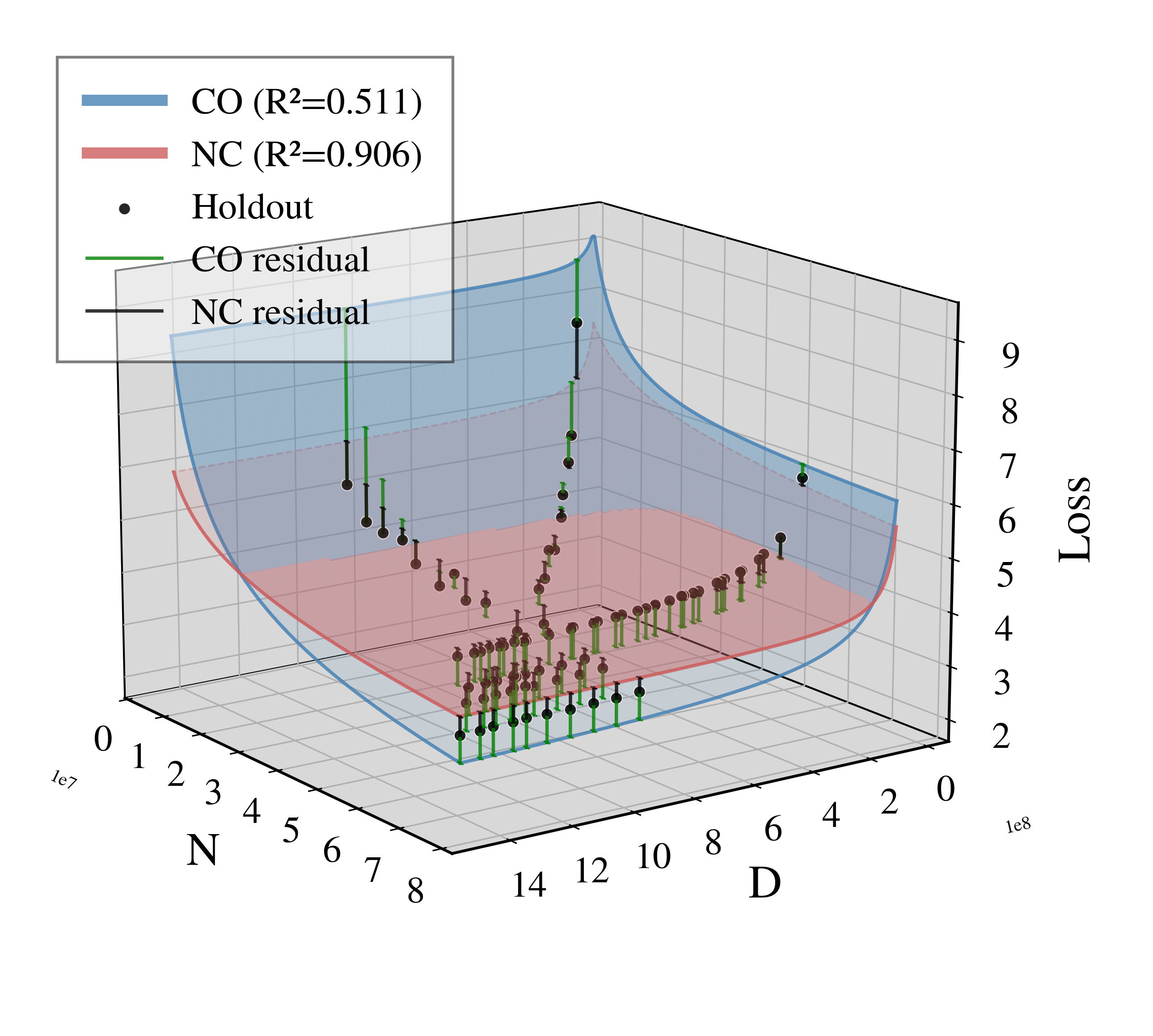
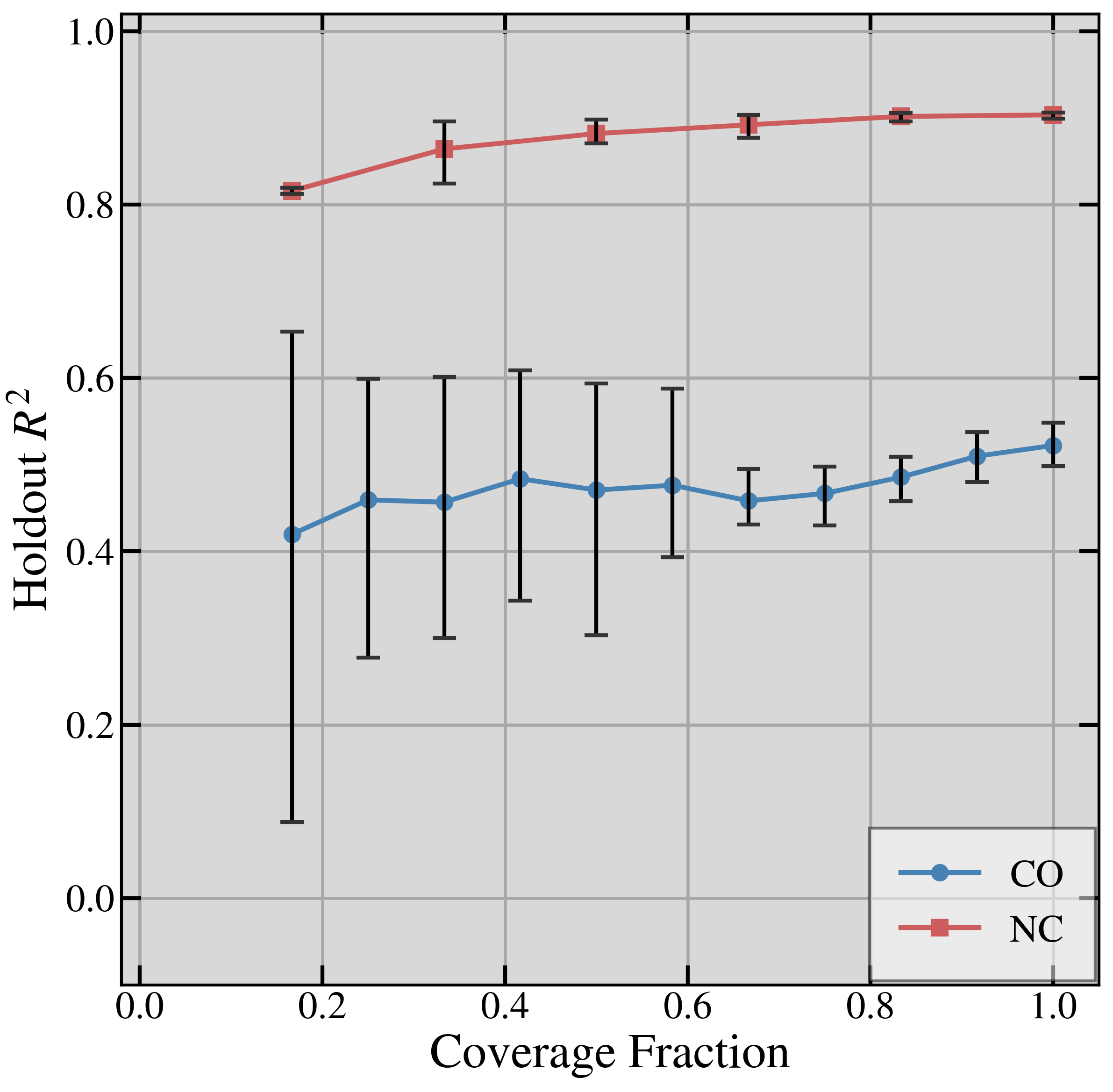
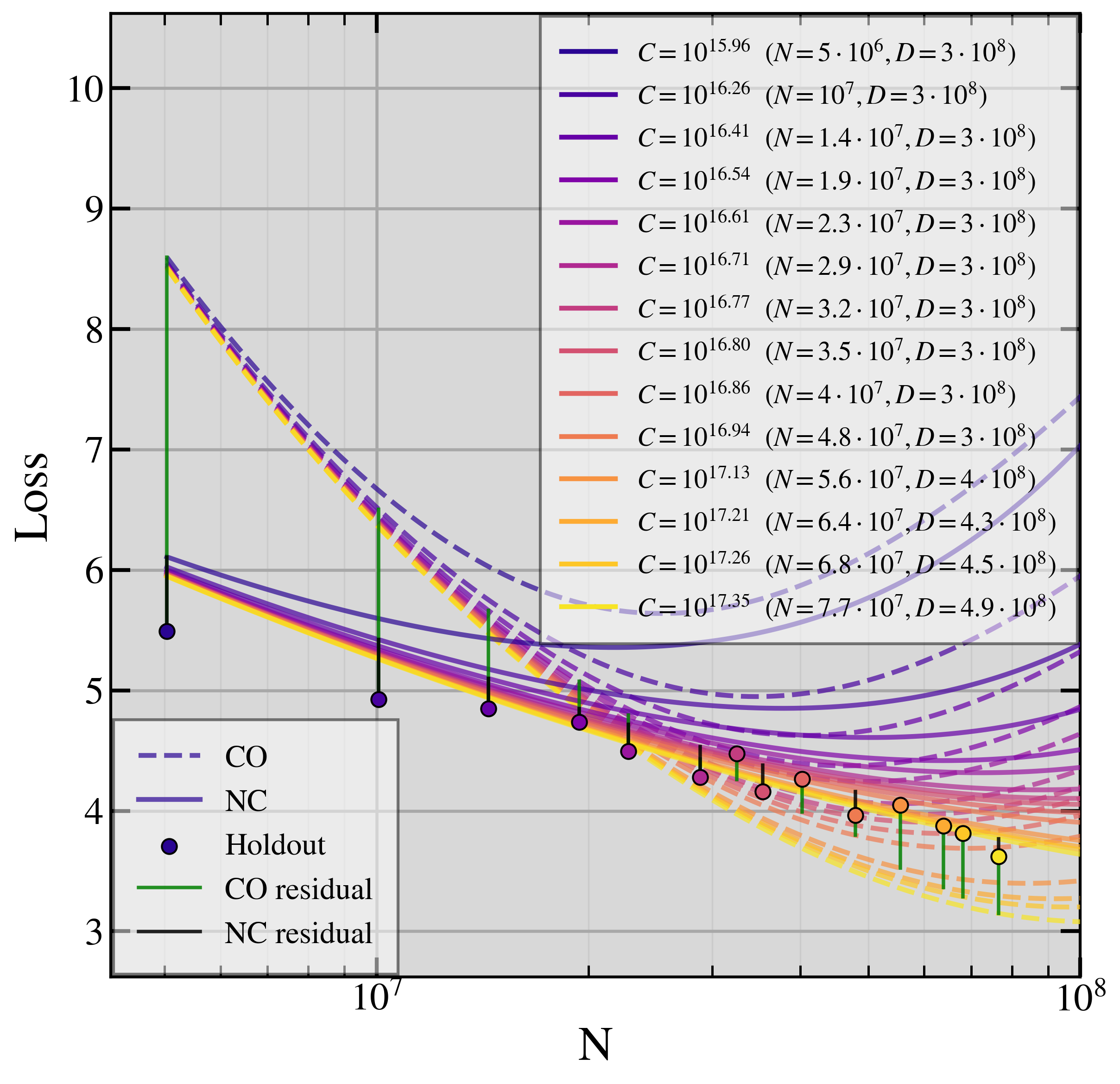
Many scaling-law studies train at one or a few fixed tokens-per-parameter ratios $k = D/N$ (a collinear design), following Chinchilla (Hoffmann et al., 2022).
On such rays the model and data terms move together, so the fit cannot tell them apart: the scale pair is ill-conditioned (a "sloppy" model; Transtrum et al., 2010; 2015), and extrapolation off the ray fails.
A closed-form threshold on the spread of the ratios, checked before training, says when a design is well conditioned.
Designs that spread runs over TPP (non-collinear) win 97.3% of extrapolation comparisons.
Abstract
Neural scaling laws approximate a language model's loss as a power-law function of parameter count $N$ and token count $D$. Following Chinchilla-style compute-optimal training, many studies fit scaling laws from runs at one or a few fixed tokens-per-parameter (TPP) ratios $k$, with $D = kN$. We show that this collinear design, combined with the empirically common near-equality of the exponents governing $N$ and $D$, induces an inherent ill-conditioning in the Gauss-Newton least-squares problem: the condition number of the design grows as the inverse square of the gap between the $N$- and $D$-exponents. The scale coefficients become practically unidentifiable, with confidence intervals inflating by orders of magnitude, yielding a "sloppy" model whose extrapolations degrade sharply off the training ray. We prove this for four scaling-law formalisms and derive a closed-form TPP-diversity threshold that characterizes well-conditioned estimation to leading order. Empirically, in controlled experiments with 5M-77M-parameter models, non-collinear designs outperform collinear ones on held-out data with a 97.3% win rate across four laws and five corpora, and 98.7% in bfloat16. We further show the degeneracy is rooted in Jacobian geometry and is not an artifact of the loss function: any smooth objective whose Gauss-Newton weights are bounded above and away from zero inherits the same ill-conditioning.
One ray cannot separate model and data
The Chinchilla rule trains at about 20 tokens per parameter, $k = D/N \approx 20$ (Hoffmann et al., 2022). On a ray $D = kN$ the Chinchilla law (Hoffmann et al., 2022) $L = AN^{-\alpha} + BD^{-\beta} + E$ becomes
$$L(N, kN) = A N^{-\alpha} + B k^{-\beta} N^{-\beta} + E,$$
so only the exponent gap $\varepsilon = |\alpha - \beta|$ separates $A$ from $B$. The scale pair's condition number grows as $\kappa_{A,B} = \Theta(\varepsilon^{-2})$, and the confidence interval on $A$ is $\Omega(\varepsilon^{-1})$ times the one on the identified combination $\psi = A + Bk^{-\alpha}$.
A threshold checkable before training
For a collinear design with ratios $k_1 < \cdots < k_K$, to leading order $\kappa_{A,B} \leq \kappa_{\mathrm{target}}$ whenever
and $\kappa_{A,B} \leq \kappa_{\mathrm{target}}$ exactly when $V_K \geq \tau_K/(1 + 1/\kappa_{\mathrm{target}})^2$. One ray never passes; two rays pass once their spread $k_2/k_1$ reaches $R_{\min}(k_1)$.
N. Muennighoff et al. Scaling data-constrained language models. JMLR 26(53), 2025. jmlr.org
M. K. Transtrum, B. B. Machta and J. P. Sethna. Why are nonlinear fits to data so challenging? Phys. Rev. Lett. 104, 2010. doi:10.1103/PhysRevLett.104.060201
M. K. Transtrum et al. Perspective: Sloppiness and emergent theories in physics, biology, and beyond. J. Chem. Phys. 143, 2015. doi:10.1063/1.4923066
BibTeX
@inproceedings{kricheli2026tpp,
  title     = {Tokens-per-Parameter Coverage Is Critical for Robust {LLM} Scaling Law Extrapolation},
  author    = {Kricheli, Joshua Shay and Reid, Alexander Lawrence and Sarkar, Soumajyoti and Gandikota, Venkata and Shakarian, Paulo},
  booktitle = {Advances in Neural Information Processing Systems},
  year      = {2026},
  note      = {arXiv:2605.08541}
}